Conditional formatting using Power BI

When you need to highlight cells based on cell value or formula within the Table or the Matrix visuals, this Power BI feature is really helpful.

Here you have the options of Background color, Font color, Data bars, and recently added KPI Icons and Web URL to customize the cells. You can either find this option by clicking the down-arrow on the column from values, based on which you want the formatting to be done or from the visualization pane formatting options.

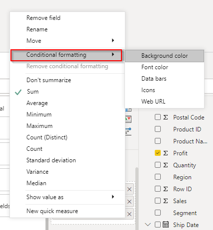
Also, have the option of removing all the formatting already been applied.

Highlight using the Background color

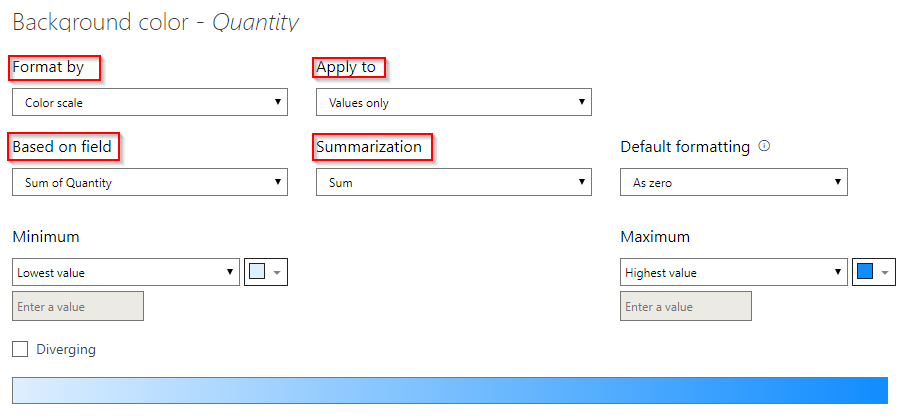
You can format the background color based on Color scale which is the basic option with simple conditions, Rules with which you can specify conditions for the data color and Field Value from the Format by category. Also, the formatting can be applied to Values, Totals, and values or Totals only. Within here it is possible to specify another column name if you want the formatting to be relative. Under the Summarization option, the type of aggregation can be selected.

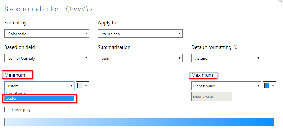
There are options to set Minimum and Maximum values as default, Lowest or Highest value, or Custom values. Next to these colors can be selected and if you check the Diverging box you will find the 3^rd option as Center value.

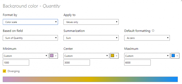
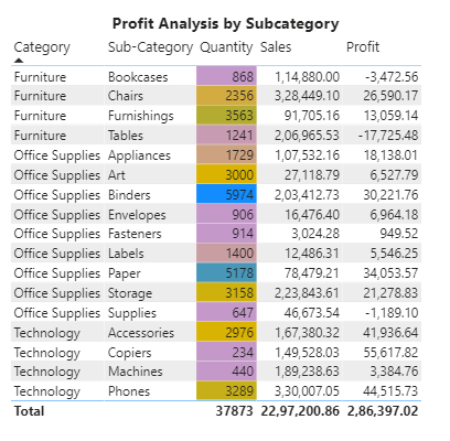
After specifying the above conditions on the Quantity column this is what I have.

Now, let’s specify some rules instead of the color scale and see how it looks.

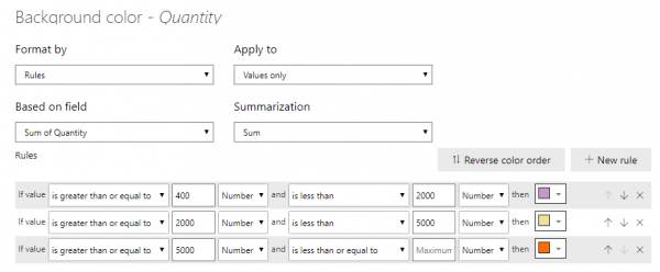
To add the rules, click on the +New rule icon. And the result is,

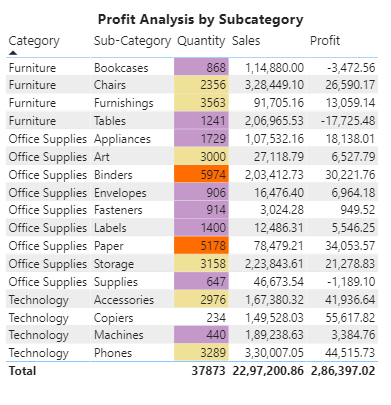
The value 234 is not in any color because I have specified the minimum value as 400.

With the Field Value option, if you have a column or measure with color name or hex value data, this feature automatically applies those colors to a column’s background or font color. You can also use custom logic to apply colors to the font or background.

Highlight using Font color

Using the font color option, let us see how the conditional formatting works.

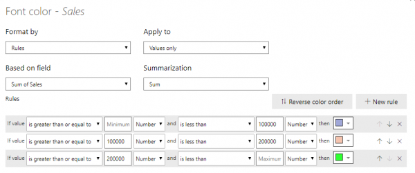
By applying rules on the Sales column this is how it looks like.

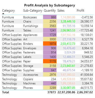
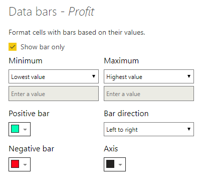
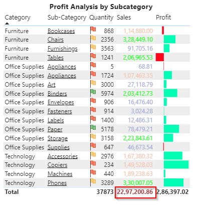
Highlight using Data bars

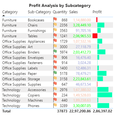
Here you have the option to see the progress of the values as bars and values or only bars. I have checked the only bars option. Indicated positive and negative bars based on the minimum and maximum values for the Profit values.

After applying the conditions, like below I have the results.

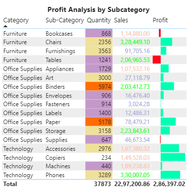
Highlight using Icons

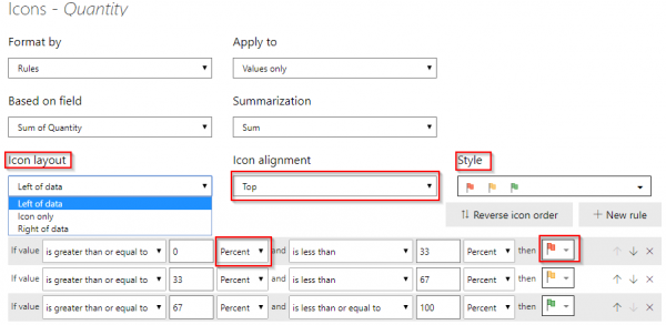
When Icons are used to highlight cell values, you can place them Top, Middle, or Bottom of the data. Within the style options, different sets of icons are available. Besides, individually you can make different combinations of icons from the icon list next to each rule. Also, it is possible to mention values as percentage or number within all the conditional formatting categories. And here is the output with Quantity values.

Highlight using Web URLs

With a column that consists of website URLs, you can use conditional formatting to apply those URLs to fields as active links.

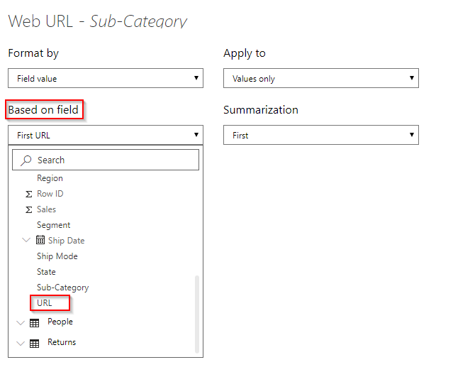
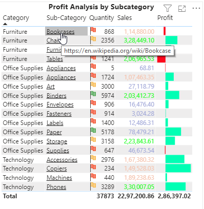
Here I have a column with URLs and I am linking this to Sub-Category column using conditional formatting. Under the Format by category, we have only the Field value category.

Now let us try Conditional formatting with Values and totals option.

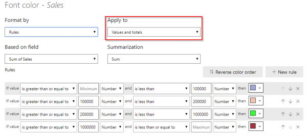
Now it has applied to the totals as well!

Please feel free to reach Cittabase for more information. Visit our blogs for more topics on Power BI.